Outline

• Motivations
• Data Visualization
• Scientific Computation
• Symbolic Computation

Motivations

• The purpose of the economic analysis is insight, not numbers.
• To learn about the intuitions behind the numbers we computed, we often need to
  • define distributions of random variables,
  • optimizing an objective function, and
  • solving a system of differential equations.

Motivations

• This chapter first introduces one of the dedicated package, namely SciPy
  • for various scientific computations.

Motivations

• Econometricians may also wish to deal with generic variables.
• We will then introduce the SymPy package,
  • which allows us perform various symbolic computations.

Motivations

• Plotting the data and the estimation results are beneficial for us to visualize the numbers.
• Matplotlib can generate plots, histograms, bar charts, scatterplots, etc.

Data Visualization: plot 2D data

• The most commonly used graph in scientific articles is the 2D plot.
• The matplotlib.pyplot is the most important command in the Matplotlib library.

Data Visualization: histogram

• We use NumPy to generate the data and apply numpy.histogram() function to create a histogram numerically.

import numpy as np
x = np.array([22,87,5,43,56,73,55,54,11,20,51,5,79,31,27])
hist,bin_edges = np.histogram(x, bins=5)
print(hist)
print(bin_edges)

[4 3 3 2 3]
[ 5.  21.4 37.8 54.2 70.6 87. ]

Data Visualization: histogram

• This function itself produces numbers but not the graph.
• Matplotlib's pyplot() sub-module can convert this numeric representation of a histogram into a chart.
• pyplot.hist() function can compute and draw the histogram as follows:

Data Visualization: histogram

from matplotlib import pyplot as plt
#引入matplotlib工具包中的pyplot模块
plt.figure(figsize=(8,5))
#设置画布大小为宽8高5
plt.hist(x, bins=5, color='gray')
#根据目标数据x画出分成5个区间的histogram
plt.title('Figure:Example of Histogram', fontsize=14)
plt.ylabel('hist', fontsize=12)
plt.xlabel('bin_edges', fontsize=12)
#设置图像的标题、y轴及x轴
plt.show()

Data Visualization: histogram

Python Tips :
在Matplotlib的线上使用手册中，将NumPy导入后并命名为np，将pyplot导入后并命名为plt。虽然导入后的命名是由代码编写者自己决定的，而np和plt的命名被更为广泛采用。在实际编程中，当代码需要发布或与他人协同编辑时，遵循普遍的命名方式会让代码更易阅读。

Data Visualization: histogram

• No plots will be displayed until the plt.show() command has been issued.
  • plt.show() command can make the window pop up and show the plot,
  • and it should be the last statement of our code.

Data Visualization: bar chart

• One can employ matplotlib.pyplot.bar() function.

x = [5,8,12]
y = [12,16,6]
plt.figure(figsize=(8,5))
# 画柱状图并且bin的标识应该位于柱状图的中心
plt.bar(x, y, align='center', color='gray')
plt.title('Figure: Example of Bar Chart', fontsize=14)
plt.ylabel(r'$y$', fontsize=12)
plt.xlabel(r'$x$', fontsize=12)
plt.show()

Data Visualization: bar chart

Data Visualization: bar chart

• align option sets the alignment of the bars to the x coordinates.

  • 'center' makes the bins to center the base on the x positions.

• In a single figure, we can also plot multiple bar charts:

Data Visualization: bar chart

x1 = [5,9,13]
y1 = [12,16,6]
x2 = [6,10,14]
y2 = [6,15,7]
x3 = [7,11,15]
y3 = [14,6,8]

plt.figure(figsize=(8,5))
plt.bar(x1, y1, align='center', color='gray', alpha=0.2)
plt.bar(x2, y2, align='center', color='gray', alpha=0.5)
plt.bar(x3, y3, align='center', color='gray', alpha=0.8)
plt.title('Figure: Example of Plotting Multiple Bar Charts',
          fontsize=14)
plt.ylabel(r'$y$', fontsize=12)
plt.xlabel(r'$x$', fontsize=12)
plt.show()

Data Visualization: bar chart

Data Visualization: scatter plot

• Seaborn is another Python data visualization library based on matplotlib.

  • and provides a high-level interface for drawing statistical graphics.

• We now make use of seaborn (a Python data visualization library based on Matplotlib) to generate the scatter plot of the Pandas data.

• The below example generates variables x and y as well as a binary indicator z. We define a variable k as a list of strings of values, either male or female.

Data Visualization: scatter plot

import random
import seaborn as sns
# 构建空的dataframe
df = pd.DataFrame()
# 在dataframe中增加列
df['x'] = random.sample(range(1,100), 10)
df['y'] = random.sample(range(1,1000), 10)
df['z'] = [1,0,0,1,0,1,0,0,1,0]
df['k'] = ['male','male','male','female',
           'female','female','male',
           'female','female','male']
# 展示输入数据后的dataframe
df

Data Visualization: scatter plot

Data Visualization: scatter plot

• seaborn.scatterplot() can be used in a way similar to Matplot functions.
• We draw a scatter plot with possibility of several semantic groupings
  • by setting the hue option.
• hue option can be used to specifiy the variable that define subsets of the data,.

Data Visualization: scatter plot

plt.figure(figsize=(8,5))
sns.scatterplot(x='x',  
           y='y',     
           data=df , # 数据源
           style="z",
           color="k")
plt.title('Figure: Example of Scatter Plot', fontsize=14)
plt.xlabel(r'$X$', fontsize=12)
plt.ylabel(r'$Y$', fontsize=12)
plt.legend(fontsize=12, framealpha=0.3)
plt.show()

Data Visualization: time series plot

• Now we use of Pandas data (i.e., Series or DataFrame) to demonstrate the time series plot and the the scatter plot.
• For the time series plot,
  • we first generate the data using pandas.date_range() function,

Data Visualization: time series plot

import pandas as pd
ts = pd.Series(np.random.randn(1000),
               index=pd.date_range('1/1/2000', periods=1000))

plt.figure(figsize=(8,5))
ts.plot(color='gray')
plt.title("Figure: Example of Time Series Data y", fontsize=14)
plt.ylabel(r"$y$", fontsize=12)
plt.xlabel("time", fontsize=12)
plt.show()

Data Visualization: time series plot

• plot() method is a convenience to plot all of them according to their column label.

y1 = np.random.randn(1000,1)+2
y2 = np.random.randn(1000,1)-2
df = pd.DataFrame(np.hstack((y1,y2)),
                  index=ts.index,
                  columns=[r"$y_1$", r"$y_2$"])

plt.figure()
df.plot(figsize=(8,5), style=[None,"--",":","-."])
plt.title("Figure: Example of Time Series Variables y1 and y2",
          fontsize=14)
plt.xlabel("time", fontsize=12)
plt.legend(loc='lower right', fontsize=12)
plt.show()

Data Visualization: line graph

• Plot the line graph for

• To generate the data, we need to compute and , coordinates of points on the curve.
• We restrict the range of in the graph to about [0,50].

x = np.arange(0,52,2)
f1 = np.sin(x)+1

Data Visualization: line graph

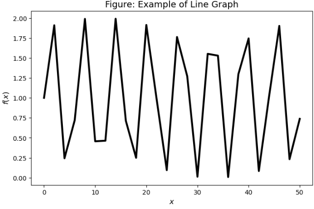
For example, to plot variable x versus variable f1:

plt.figure(figsize=(8,5))
plt.plot(x, f1, 'k-', lw=3)
plt.title('Figure: Example of Line Graph', fontsize=14)
plt.xlabel(r'$x$', fontsize=12)
plt.ylabel(r'$f(x)$', fontsize=12)
plt.show()

Data Visualization: line graph

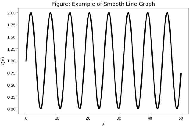
• The above plot is quite kinked.
• Consider the improved code:

x = np.arange(0,50.2,0.2)
f1 = np.sin(x)+1

plt.figure(figsize=(8,5))
plt.plot(x, f1, 'k-', lw=3)
plt.title('Figure: Example of Smooth Line Graph', fontsize=14)
plt.xlabel(r'$x$', fontsize=12)
plt.ylabel(r'$f(x)$', fontsize=12)
plt.show()

Data Visualization: line graph

Data Visualization: line graph

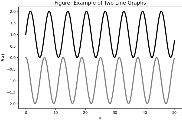
Also, we can add another line graph of function the to above existing plot:

f2 = np.cos(x)-1

plt.figure(figsize=(8,5))
plt.plot(x, f1, 'k-', lw=3)
plt.plot(x, f2, 'gray', lw=3)
plt.title('Figure: Example of Two Line Graphs', fontsize=14)
plt.xlabel(r'$x$', fontsize=12)
plt.ylabel(r'$f(x)$', fontsize=12)
plt.show()

Data Visualization: line graph

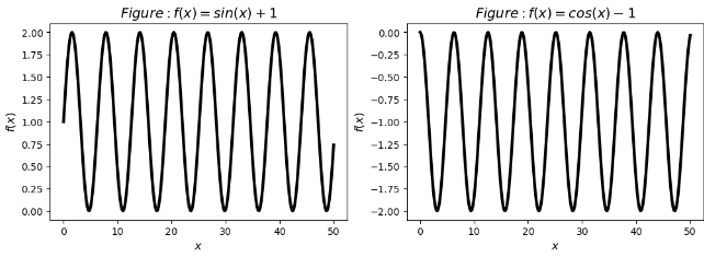
Alternatively, we can plot two functions in two subplots of a same figure.

plt.figure(figsize=(12,8))

plt.subplot(2,2,1)
plt.plot(x, f1, 'k-', lw=3)
plt.title('$Figure: f(x)=sin(x)+1$', fontsize=14)
plt.xlabel(r'$x$', fontsize=12)
plt.ylabel(r'$f(x)$', fontsize=12)

Data Visualization: line graph

# 指定subplot的尺寸构图为2行2列当中的第2个图
plt.subplot(2,2,2)
plt.plot(x, f2, 'k-', lw=3)
plt.title('$Figure: f(x)=cos(x)-1$', fontsize=14)
plt.xlabel(r'$x$', fontsize=12)
plt.ylabel(r'$f(x)$', fontsize=12)
# 展示图片
plt.show()

Data Visualization: fine tuning the plot

• One might wish to add proper
  • titles,
  • labels,
  • captions,
  • and legends to the graph.
• See below example.

Data Visualization: fine tuning the plot

# 图片格式微调
plt.figure(figsize=(8,5))
plt.title("Figure: Title of the figure",
          fontsize=14) # 图像的全称
plt.xlabel(r"$x$", fontsize=12)   
plt.ylabel(r"$f(x)$", fontsize=12) 
plt.plot(x, f1, label="$sin(x)+1$",
         color="k",
         linewidth=1)
plt.plot(x, f2, label="$cos(x)-1$", color="gray",
         linewidth=3, linestyle="dotted")
plt.legend(fontsize=12) 
plt.grid()   # 在图像当中输出网格分割线
plt.show()   # 在图像当中将目标图像画出

Data Visualization: fine tuning the plot

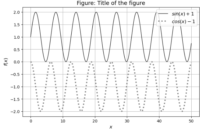
• figsize=(8,4) restricts the figure size to 8 by 4 inches.
• label defines the name of this line and will in the legend().
• legend() displays a legend with the labels.
• grid() displays a grid on the backdrop.
• plt.plot we can choose the line style, thickness, color, etc.

Data Visualization: fine tuning the plot

• More in-depth guides for using Matplotlib:
  • matplotlib.org/stable/tutorials/index.html
• Extended thumbnail gallery of examples:
  • matplotlib.org/stable/gallery/index.html

Scientific Computation

• SciPy (SCIentifc Python) library provides algorithms for
  • optimization,
  • integration,
  • interpolation,
  • eigenvalue problems,
  • algebraic equations,
  • differential equations,
  • statistics,
  • and many other classes of problems.

Scientific Computation

• SciPy is built on NumPy,
  • and it extends NumPy providing additional tools for array computing and specialized data structures.
• Note that many functions from NumPy are available in SciPy as well.

Scientific Computation: optimization toolbox

• SciPy has a very powerful optimization toolbox
  • it has several commonly used optimization algorithms.
• We next introduce
  1. the roots-finding tools
  2. and the routine for optimization.

Scientific Computation: roots-finding

• First, we introduce the bisection (bisect()) algorithm, which is robust and conceptually simple.
• Suppose we want to find roots of .
• bisect() method takes three compulsory arguments:
  • f: the function ,
  • a lower limit a,
  • and an upper limit b.

Scientific Computation: roots-finding

Clearly, would have roots at and at .

from scipy.optimize import bisect
def f(x):
    return x**3 - 2 * x**2

x1 = bisect(f, a=-1, b=0)
x2 = bisect(f, a=1.5, b=3)
x1,x2

(0.0, 1.9999999999995453)

Scientific Computation: roots-finding

• fsolve method can be applied for more general purposes,
  • such as multidimensional functions.
• fsolve algorithm needs only one starting point (x0 option) close to the suspected location of the root.

from scipy.optimize import fsolve
x1 = fsolve(f, x0=0)
x2 = fsolve(f, x0=2)
x1, x2

 (array([0.]), array([2.]))

Scientific Computation: optimizing a function

• Optimizing a function is one of the most critical tasks in most statistical and econometric applications.
• In SciPy, fmin() and minimize() methods can perform such tasks.

Scientific Computation: optimizing a function

• scipy.optimize.fmin() command and try to maximize a simple function to find

from numpy import arange,cos,exp
from scipy.optimize import fmin
def f(x):
    return cos(x) - 3*exp(-(x-0.2)** 2)

Scientific Computation: optimizing a function

x = arange(-20,20,0.1)
y = f(x) # Note, -f(x) = g(x)

plt.figure(figsize=(8,5))
plt.plot(x, y, 'k-', lw=3)
plt.title('Figure: Inspect the Function $f(x)=\cos(x) - 3\exp[-(x-0.2)^2]$', fontsize=14)
plt.xlabel(r'$x$', fontsize=12)
plt.ylabel(r'$f(x)$', fontsize=12)
plt.grid()
plt.show()

Scientific Computation: optimizing a function

• scipy.optimize.fmin(f,x0) function takes two arguments:

  1. The function f to minimize
  2. and an initial value x0 from which to start the search.

• It returns the value x for which f(x) is locally minimized.

Scientific Computation: optimizing a function

• The search for the minimum is a local search around the starting point,
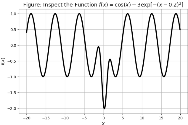
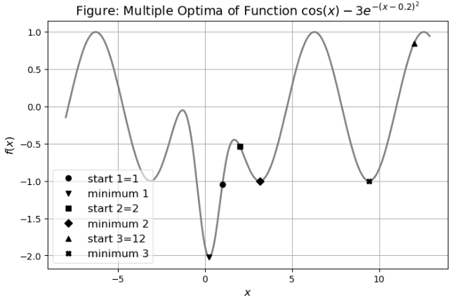
• The above plot shows that setting different starting points (e.g. x0=2 or x0=12) might be failed to find the global minima.
• See the below code for inspection.

Scientific Computation: optimizing a function

# 从1,2,12开始，分别寻找f(x)的最小值
minimum1 = fmin(f, 1.0) 
print("Start search at x=1, minimum is",minimum1)
minimum2 = fmin(f, 2.0) 
print("Start search at x=2, minimum is",minimum2)
minimum3 = fmin(f, 12.0) 
print("Start search at x=12, minimum is",minimum3)

Optimization terminated successfully.
         Current function value: -2.023866
         Iterations: 16
         Function evaluations: 32
Start search at x=1, minimum is [0.23964844]
Optimization terminated successfully.
         Current function value: -1.000529
         Iterations: 16
         Function evaluations: 32
Start search at x=2, minimum is [3.13847656]
Optimization terminated successfully.
         Current function value: -1.000000
         Iterations: 17
         Function evaluations: 34
Start search at x=12, minimum is [9.42480469]

Scientific Computation: optimizing a function

• scipy.optimize.minimize(f,x0) function has a similar syntax
  • for compulsory arguments and can generate (almost) identical results:

from scipy.optimize import minimize
minimize(f, 1.0).x, minimize(f, 2.0).x, minimize(f, 12.0).x

(array([0.23961728]), array([3.13845708]), array([9.42477932]))

Scientific Computation: optimizing a function

For different starting values:

x = arange(-8,13,0.1)
y = f(x)

plt.figure(figsize=(8,5))
plt.plot(x, y,'gray',lw=2)
plt.title('Figure: Multiple Optima of Function $\cos(x)-3e^{ -(x -0.2)^2}$', fontsize=14)
plt.xlabel(r'$x$', fontsize=12)
plt.ylabel(r'$f(x)$', fontsize=12)
plt.grid()

plt.plot(1.0 ,f(1.0), 'ok', label ='start 1=1')
plt.plot(minimum1, f(minimum1), 'vk', label='minimum 1')

plt.plot(2.0, f(2.0), 'sk', label='start 2=2')
plt.plot(minimum2, f(minimum2), 'Dk', label='minimum 2')

plt.plot(12.0 ,f(12.0), '^k', label='start 3=12')
plt.plot(minimum3, f(minimum3), 'Xk', label='minimum 3')

plt.legend(loc='lower left', fontsize=12, framealpha=0.6)
plt.show()

Scientific Computation: probability distributions

• All of the statistics functions are located in the sub-package scipy.stats.
• It contains a large number of probability distributions.

Scientific Computation: uniform distributions

For the PDF of a uniform distribution

from scipy.stats import uniform
uniform.pdf([0,1,2,3,4], loc=0, scale=1)

array([1., 1., 0., 0., 0.])

Scientific Computation: Normal distributions

• For the normal distribution, we can use the norm(loc,scale) function to implement.
  • The loc (location) keyword specifies the mean,
  • and the scale keyword specifies the standard deviation.
• Consider the following example:

Scientific Computation: Normal distributions

from scipy.stats import norm
norm.pdf(np.array([0,-1,1,-200,100]))

array([0.39894228, 0.24197072, 0.24197072, 0.        , 0.        ])

Scientific Computation: Normal distributions

norm.cdf(np.array([0,-1,1,-2,10]))

array([0.5       , 0.15865525, 0.84134475, 0.02275013, 1.        ])

Scientific Computation: Normal distributions

To find the q-th quantile of a distribution, we can use the Percent Point Function (norm.ppf(q)):

norm.ppf(0.5)

0.0

Scientific Computation: Normal distributions

The median can also be found using median method directly:

norm.median(loc=0, scale=1)

0.0

Scientific Computation: Normal distributions

Similarly, mean, var and std functions give the mean, variance, and standard deviation of the distribution.

print( "Mean of N(5,10) is %2.1f"
     % (norm.mean(loc=5, scale=10)))
print( "Variance of N(5,10) is %2.1f"
     % (norm.var(loc=5, scale=10)))
print( "Standard deviation of N(5,10) is %2.1f"
     % (norm.std(loc=5, scale=10)))

Mean of N(5,10) is 5.0
Variance of N(5,10) is 100.0
Standard deviation of N(5,10) is 10.0

Scientific Computation: Normal distributions

To generate a sequence of random normal variates:

norm.rvs(0, 10, size=4)

array([-21.50986762,  -5.84663993,   6.56998426,  11.75718474])

To generate the same random numbers, use the seed function.

Scientific Computation: Normal distributions

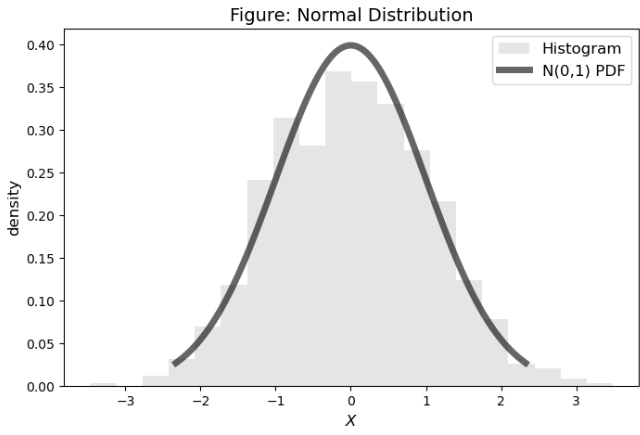
plt.figure(figsize=(8, 5))
# Histogram
plt.hist(norm.rvs(0, 1, size=1000), bins=20, alpha=0.2,
         density=True, color='gray', label='Histogram')
# PDF
x = np.linspace(norm.ppf(0.01), norm.ppf(0.99), 100)
plt.plot(x, norm.pdf(x), 'k-', lw=5, alpha=0.6,
         label='N(0,1) PDF')
plt.title('Figure: Normal Distribution', fontsize=14)
plt.xlabel(r'$X$', fontsize=12)
plt.ylabel('density', fontsize=12)
plt.legend(loc='best', fontsize=12)
plt.show()

Scientific Computation: Poisson distributions

• Poisson distribution can be implemented respectively using poisson object.
• For example, suppose that the average number of patients visiting a hospital is 3 per hour.
• Then, the probability that 6 patients visit the hospital in a given hour is .

from scipy.stats import poisson
poisson.pmf(k=6, mu=3)

0.05040940672246224

Scientific Computation: binomial distributions

• The Poisson distribution is closely related to the binomial distribution.
• For the binomial distribution, binom function takes n and p as shape parameters, where n is the number of trails and p is the probability of a single failure.

from scipy.stats import binom
binom.pmf(k=5, n=10, p=0.4, loc=1)

0.25082265599999987

Scientific Computation: binomial distributions

Note that binom.pmf(k, n, p, loc) is identically equivalent to binom.pmf(k - loc, n, p).

binom.pmf(k=5-1, n=10, p=0.4, loc=0)

0.25082265599999987

Scientific Computation: exponential distribution

The expon function in scipy.stats is for the exponential distribution. E.g.,

from scipy.stats import expon
expon.cdf(x=10, loc=0, scale=5)

0.8646647167633873

Scientific Computation: quadrature

• quad() (stands for quadrature) function in the scipy.integrate module performs the numerical integration of the kind

• quad() function takes arguments of
  • integrand ,
  • and the lower and upper limits and .
• Consider

Scientific Computation: quadrature

import scipy
from math import cos, exp, pi
from scipy.integrate import quad
# 定义我们需要积分的函数
def f(x):
    return(exp(cos(-2*x*pi) + 3.2))

result, error = quad(f,-2,2)
print("The numerical result is %f (+- %g)" % (result,error))

The numerical result is 124.239198 (+- 3.80539e-10)

Scientific Computation: quadrature

• quad returns a tuple with two values:
  • the computed results,
  • and the numerical error of the result.

print(quad(f, -2, 2, epsabs=1))
print(quad(f, -2, 2, epsabs=1.5e-25))

(124.23919750991882, 0.0004461052678550459)
(124.23919750992361, 3.805389029468099e-10)

Scientific Computation: ODE

• We use odeint function to solve an ordinary differential equation of the type
  

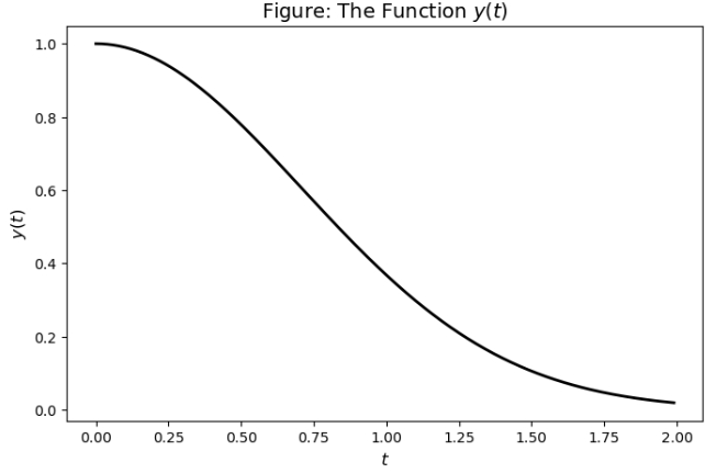
• Consider the example finds for with initial value given the equation .

Scientific Computation: ODE

from scipy.integrate import odeint
# 定义ODE
def f(y,t):
    return -2*y*t
# Initial value 起始值
y0 = 1
# 积分区间
a = 0
b = 2
# 定义t的值
t = np.arange(a,b,0.01)
# 利用odeint()函数实现
y = odeint(f, y0, t)

Scientific Computation: ODE

plt.figure(figsize=(8,5))
plt.plot(t, y,'k-',lw=2)
plt.title(r'Figure: The Function $y(t)$', fontsize=14)
plt.xlabel(r'$t$', fontsize=12)
plt.ylabel(r'$y(t)$', fontsize=12)
plt.show()

Symbolic Computation

• The symbolic computation method
  • Python using the SymPy (SYMbolic Python) library.
• The SymPy home page is sympy.org, and provides the up-to-date documentation for this library.

Symbolic Computation: undefined variables

Create symbolic variables using SymPy’s Symbol function:

import sympy
x = sympy.Symbol('x')
y = sympy.Symbol('y')
y - x + y + 10 * y**6

Symbolic Computation: undefined variables

Variables with subscription (and in Greek letters) can also be defined:

x1 = sympy.Symbol('x_1')
x2 = sympy.Symbol('x_2')
alpha1 = sympy.Symbol('alpha_1')
rho2 = sympy.Symbol('rho_2')
Sigma =  sympy.Symbol('Sigma_n')
x1 + x2 + alpha1 + Sigma  + rho2

Symbolic Computation: variables and functions

We can abbreviate the creation of multiple symbolic variables using the symbols function.

x,y,z = sympy.symbols('x,y,z')
equation = x + 2/y*z + z**2
equation

Symbolic Computation: variables and functions

Btw, latex() function converts results to latex code:

sympy.latex(equation) # 把符号转换为TeX代码

'x + z^{2} + \\frac{2 z}{y}'

Symbolic Computation: variables and functions

To insert real numerical values instead of generic variables:

x,y = sympy.symbols('x,y')
(x + 2*y).subs(x, 10)

Symbolic Computation: variables and functions

(x + 2*y).subs(x, 10).subs(y, 3)

We can also substitute a symbolic variable for another one by:

myterm = 3*x + y**2
myterm.subs(x, y).subs(y, 2)

Symbolic Computation: undefined Functions

Define a symbolic function using Function method:

x,y,theta,n = sympy.symbols('x,y,theta,n')
l = sympy.Function('l')(x,y,theta,n)
l

Variables can be defined after generating the function:

g = sympy.Function('g')
g(x,y,theta,n)

Symbolic Computation: solving for roots

• For example, solve
  
• We use the root solver within the solvers.

x = sympy.symbols('x')
sympy.solvers.solve(x**2 - 2*x)

[0, 2]

Symbolic Computation: solving for roots

• Another example is solving .
• Multiple roots can be found.

def f(x):
    return x**3 - 2*x - 5
sympy.solvers.solve(f(x))

[(-1/2 - sqrt(3)*I/2)*(sqrt(1929)/18 + 5/2)**(1/3) + 2/(3*(-1/2 - sqrt(3)*I/2)*(sqrt(1929)/18 + 5/2)**(1/3)),
 2/(3*(-1/2 + sqrt(3)*I/2)*(sqrt(1929)/18 + 5/2)**(1/3)) + (-1/2 + sqrt(3)*I/2)*(sqrt(1929)/18 + 5/2)**(1/3),
 2/(3*(sqrt(1929)/18 + 5/2)**(1/3)) + (sqrt(1929)/18 + 5/2)**(1/3)]

Symbolic Computation: differentiation

• In economics,
  • researchers are interested in marginal utility based on estimation results.
  • This requires us to take (partial) derivatives.
• Consider diff(function, variable) function:

Symbolic Computation: differentiation

x,y,z = sympy.symbols('x,y,z')
sympy.diff(2*x, x)

sympy.diff(10 + 3*x + 4*y**2 + 10* x**2 + x**9 , y)

Symbolic Computation: differentiation

• Note that SymPy provides simple math functions such as , and for symbolic computation.
• For example:

sympy.diff(10 + 3*x + 4*y**2 + 10* x**2 + x**9 , y).subs(y, 2)

Symbolic Computation: differentiation

For higher derivatives:

sympy.diff(3*x**4, x)

Symbolic Computation: differentiation

sympy.diff(3*x**4, x, x)

sympy.diff(3*x**4, x, x, x)

For the partial derivative with respect to different variables:

sympy.diff(sympy.diff(x**2 * y**7, x), y)

Symbolic Computation: integration

The integration uses a similar syntax.

x,y = sympy.symbols('x,y')
sympy.integrate(x**2, x) # 积分方程X^2

sympy.integrate(x**2, (x, 0, 1))

Symbolic Computation: Taylor expansions

• Taylor expansion is a vital math technique for many aspects of the econometric theory.
• It is possible to expand many SymPy expressions as the Taylor series.
• The basic syntax is sympy.series(expression, x=None, x0=0, n=6).

x = sympy.Symbol('x')
# 对方程sin(x) 关于x在x=0的附近展开
sympy.series(sympy.sin(x), x, x0=0)

Symbolic Computation: Taylor expansions

We can also specify
- the point around which to expand (x0=0 by default),
- the maximum term number by option n,
- and the direction of the expansion.

sympy.series(sympy.sin(x), x, x0=0, n=10)

Symbolic Computation: Taylor expansions

x0 = sympy.Symbol('x_0')
sympy.series(sympy.sin(x), x, x0, 5)

Symbolic Computation: Taylor expansions

One might wish to discard the big-O term:

sympy.series(sympy.sin(x), x, x0, 5).removeO() # 对方程sin(x) 关于x在x0的附近展开,并且最高次项等于5并且去掉大O项

Symbolic Computation: probability distributions

• sympy.stats sub-module introduces a random variable type into the SymPy.
  • It has functions such as Normal and Exponential.
• We use both univariate and multivariate normal distributions as examples.

Symbolic Computation: univariate Normal variable

The normally distributed variable can be defined using Normal(X, mean, std)

from sympy.stats import *
x = sympy.Symbol('x')
X = Normal("X", 0, 1) # 定义变量X服从mean为0，sd为1的正态分布

And its pdf. and cdf. can be seen:

density(Normal("X", 0, 1))(x) # 变量X的pdf

Symbolic Computation: univariate Normal variable

P(X <= 0) # 变量X小于0的概率

P(X < x) # 变量X小于x的概率

Symbolic Computation: univariate Normal variable

For the expectation and variance quantities:

E(X), variance(X*8+5)

(0, 64)

Symbolic Computation: multivariate Normal variable

• Define and as two independent standard variables.
• is the sum of two marginal variances.

X = Normal("X", 0, 1)
Y = Normal("Y", 0, 1)
variance(X+Y)

Symbolic Computation: multivariate Normal variable

• Can we allow the correlation between and ?
  • The answer is yes.
• Consider a vector of two random variables ,
• We use MatrixSymbol method to define a

Symbolic Computation: multivariate Normal variable

Z = sympy.MatrixSymbol('Z', 2, 1)

We must specify the variance-covariance matrix using SymPy.

sympy.Identity(2).as_explicit()
Z = (Normal("Z", [0,0], sympy.Identity(2).as_explicit()) )
variance(Z[0]+Z[1])

Symbolic Computation: multivariate Normal variable

For the density function:

z = sympy.MatrixSymbol('z', 2, 1)
density(Z)(z)

Symbolic Computation: multivariate Normal variable

• If we define the covariance of 0.2,
• we can find the the variance of can be computed according to:

Cov = sympy.Matrix([[1,0.2],[0.2,1]])
Z = (Normal("Z", sympy.Matrix([0, 0]), Cov))
variance(Z[0]+Z[1])